

pass and fail. It’s the same flow as the video, but slower and with screenshots — a good first run if you’re new to the platform.
By the end you’ll have a trained model deployed to a device and catching defects on a live video feed.
Before you start
You’ll need an AcuSight account and some images to work with — either an edge device that’s streaming images, or a folder of images on your computer. No local install required.Step 1 — Create a project and bring in images
Open Projects and create one — call it Cable glands. A project is the workspace that ties your images, dataset, and models together. Then add images:- From a device — images your devices capture arrive automatically as batches. Open a batch and choose Move Batch to Project. If you haven’t provisioned a device, see Connect a device.
- Upload — use Upload Data to add a folder straight from your computer.
Step 2 — Annotate
Open Annotate. Your batch starts under Unassigned — open it to begin labeling. Draw a box around each part and assign it a class:pass or fail. You manage classes and their colors on Classes & Tags.
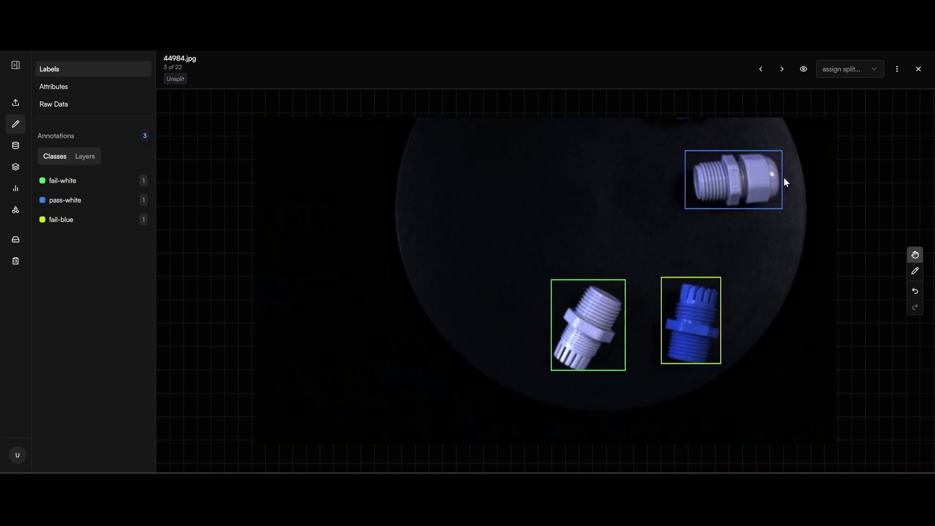
Draw a box around each part and assign it a class as you work through the batch.
Step 3 — Freeze a dataset version
Once enough images are labeled, add them to the dataset and pick a train / validation / test split. Then open Snapshots → Create Snapshot to freeze an immutable dataset version — the exact set of images and labels your model will learn from. Optionally add:- Preprocessing — for example, drop un-annotated images.
- Augmentation — for example, horizontal flips, to help the model generalize.
Step 4 — Train
Choose Train Model on your dataset version. Pick an architecture — YOLOv8 is a solid default — and a size. Nano trains fast and runs well on edge devices.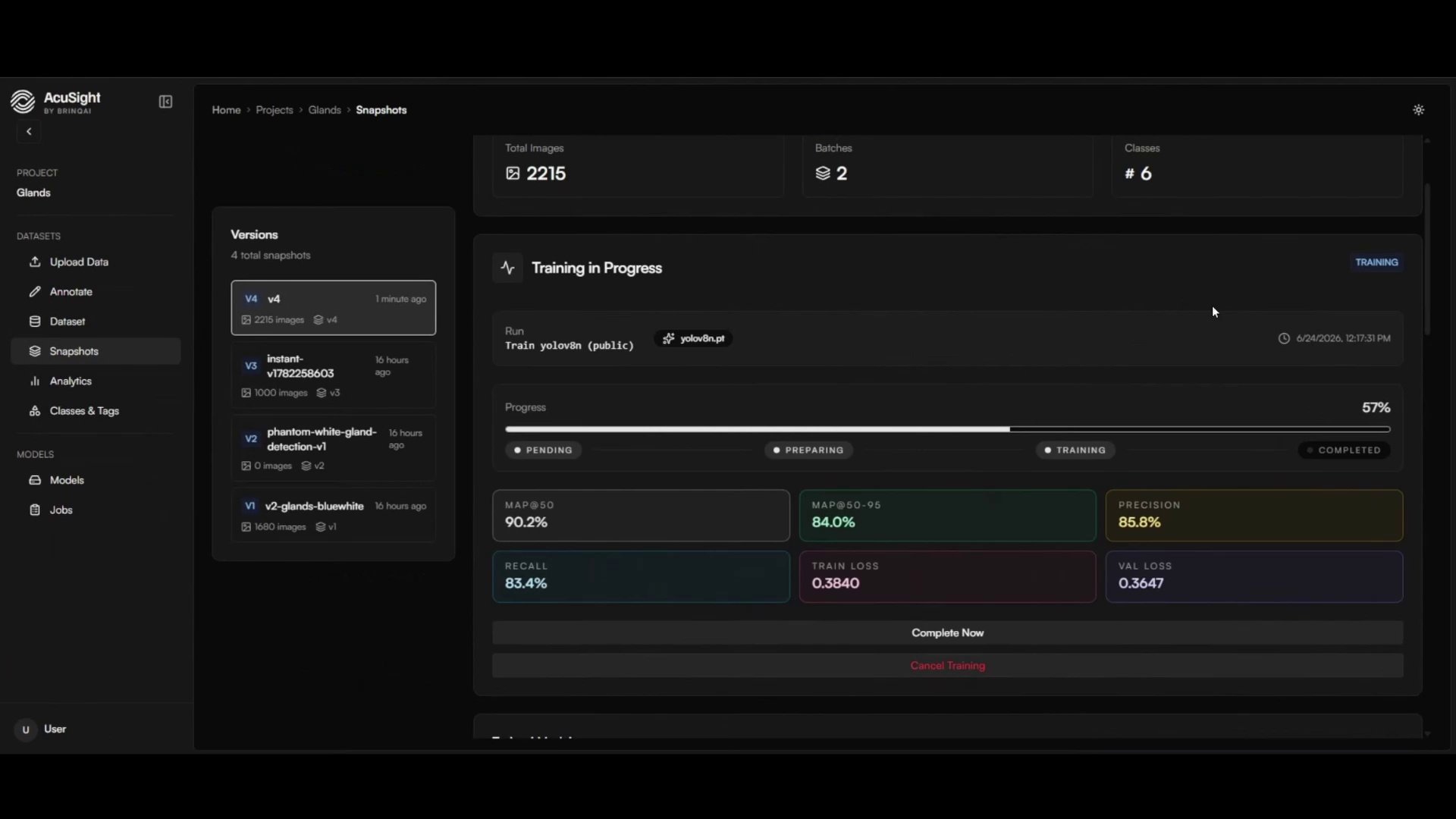
Accuracy and loss metrics stream in live as training runs.
Step 5 — Evaluate and promote
Before deploying, check the model actually holds up. On the model’s page, review its metrics against the test split — the data it never trained on. When a model beats your current best, promote it to champion so it becomes the one that ships. See Model eval & champion promotion.Step 6 — Deploy and watch it run
Open Models, select your model, and choose Deploy, then pick the group to deploy to. Every device in it picks up the model on its next check-in. Open the Video tab to watch live inference — detections appear in real time, with Good / Defect events listed alongside.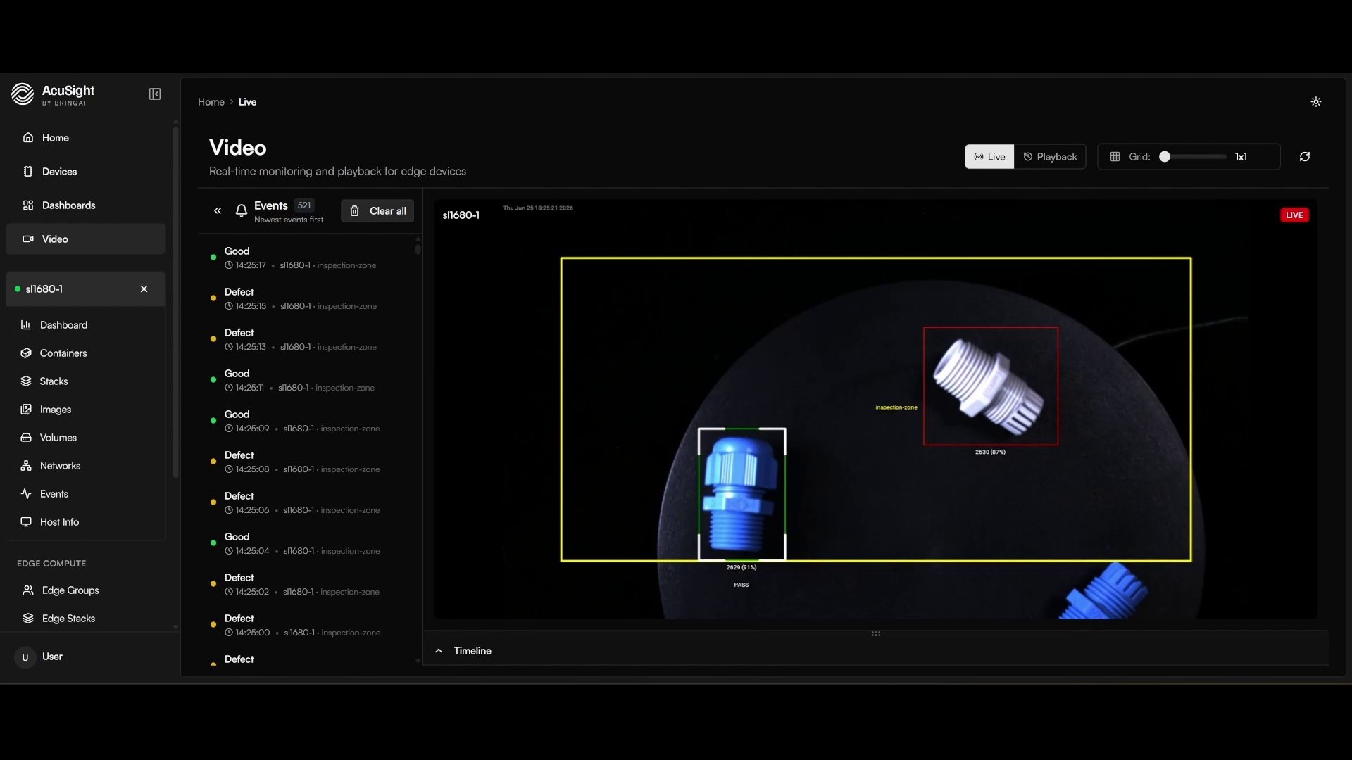
Live inference on the device — detections and pass/fail events in real time.
Keep it accurate over time
Parts change and new defects appear. Adapting the model is the same path you just walked: collect more images, re-annotate, snapshot, retrain, and redeploy. Because every model is tied to an immutable dataset version, you can always compare a new model against the one it’s replacing.Next steps
Run it across a fleet
Deploy this model to many devices and manage them as one.
Ask the Co-Pilot
Check on your data, models, and detections in plain English.